10 Excel 2013 Advanced Formulas and Functions: Power Moves for Data Crunchers

Struggling with nested formulas that clutter your spreadsheet? Array formulas in Excel 2013 let you perform multiple calculations in a single cell—no more stacking IF statements or convoluted logic. Unlike traditional formulas, they process entire ranges of data at once, making them perfect for financial modeling, dynamic reporting, and complex data analysis.

To use them, simply enter your formula (e.g., {=SUM(A1:A10*B1:B10)}) and press Ctrl+Shift+Enter to activate the curly braces. Excel 2013 supports CSE (Control+Shift+Enter) array formulas, which are ideal for tasks like calculating moving averages, conditional sums, or multi-criteria lookups without helper columns. For example, {=SUM(IF(A2:A100="Yes",B2:B100))} sums only values where column A matches "Yes"—all in one cell!

This is a game-changer for financial analysts, data scientists, and report builders who need clean, efficient spreadsheets. Start with simple array formulas, and you’ll wonder how you ever worked without them. ✨

Tired of VLOOKUP’s limitations—like rigid column positions or #N/A errors? The INDEX-MATCH duo replaces it with a dynamic, error-free powerhouse that works left-to-right, top-to-bottom, or even with multiple criteria.

Here’s how it works: INDEX locates the exact cell (row and column), while MATCH finds the lookup value’s position. Combine them like =INDEX(returnrange, MATCH(lookupvalue, lookup_range, 0)) to pull data from any direction—no column-order dependency. This combo also handles multi-criteria lookups (e.g., matching both product and region) without nested IFs.

Perfect for analysts juggling large datasets (think inventory, sales, or HR records) where VLOOKUP’s quirks cause headaches. Once mastered, it’s the go-to for zero-config flexibility. ✨

Tired of manually filtering data just to get a simple sum? SUMIFS and SUMIF let you add up values based on one or multiple conditions—no pivot tables required. Whether you're tracking sales by region and product category or calculating inventory costs for specific suppliers, these functions cut hours of manual work down to seconds.

SUMIF handles single criteria (e.g., sum all orders from "Region West"), while SUMIFS (note the "S") lets you stack conditions (e.g., sum orders from "Region West" and "Product A" and "Q2 2013"). Both support wildcards for partial matches, making them perfect for messy real-world data. Excel 2013 even lets you reference entire columns directly, so your formulas stay dynamic as your data grows.

Accountants, retail managers, and operations teams will love how these functions replace clunky nested IFs or helper columns. Start with SUMIF for simple filters, then graduate to SUMIFS when your criteria get complex—your spreadsheets (and sanity) will thank you. ✨

Tired of struggling with inconsistent text data in Excel? TEXTJOIN and TRIM are your secret weapons for cleaning up messy datasets effortlessly. Whether you're merging customer lists, standardizing product names, or preparing data for exports, these functions save hours of manual work.

TEXTJOIN combines text from multiple cells into one, ignoring empty cells and adding a delimiter of your choice—like commas or spaces. Pair it with TRIM to remove extra spaces from text, ensuring uniformity. For example, =TEXTJOIN(", ", TRUE, TRIM(A2:A10)) merges cells A2 to A10 with commas, skipping blanks and trimming whitespace. These functions work seamlessly in Excel 2013, making them perfect for legacy systems still in use.

Ideal for marketers, data analysts, or anyone dealing with raw text imports, these tools turn cluttered data into polished, export-ready formats with minimal effort. ✨

Tired of manually counting workdays or guessing end-of-month deadlines? The EOMONTH and NETWORKDAYS functions in Excel 2013 are your secret weapons for precise date calculations.

EOMONTH instantly finds the last day of any month—whether you’re calculating quarterly reports or payroll cycles. For example, =EOMONTH("5/15/2023", 2) returns June 30, 2023, without manual adjustments. Meanwhile, NETWORKDAYS counts only actual workdays (excluding weekends and holidays), perfect for project timelines or vacation planning.

Ideal for HR teams managing payroll schedules, project managers tracking milestones, or operations staff planning deadlines, these functions save hours of guesswork. ⚡

Ever opened an Excel workbook only to be greeted by a sea of #DIV/0! or #N/A errors? IFERROR and ISERROR are your secret weapons to turn those red flags into clean, professional results—without rewriting your entire formula.

Use IFERROR(value, valueiferror) to display a custom message when a formula fails (e.g., show "N/A" instead of #N/A!). Pair it with ISERROR(test) for conditional logic—like checking if a division result is valid before proceeding. These functions work in Excel 2013 and later, making them perfect for automated reports where errors could derail analysis.

Accountants auditing financial statements and team leads distributing shared dashboards will appreciate how these functions keep workbooks running smoothly. No more frustrated users or last-minute fixes—just polished, error-free outputs. ✨

Tired of manually adjusting cell references every time your dataset grows? The OFFSET and INDIRECT combo lets you build self-adjusting ranges that expand or contract automatically—no more broken formulas when you add new rows or columns.

With OFFSET, you define a starting point and specify how many rows/columns to shift (e.g., =OFFSET(A1,1,2)). Pair it with INDIRECT to turn text into dynamic references (e.g., =INDIRECT("A"&ROW())), making ranges like =SUM(INDIRECT("Sales!"&A1&":Sales!"&B1)) update seamlessly. This is a game-changer for rolling reports or dashboards where data ranges fluctuate.

Perfect for analysts managing variable-length datasets—like monthly sales reports or inventory logs—where rigid cell references would break. ⚡

Tired of basic averages that hide critical insights in your datasets? AVERAGEIFS and PERCENTRANK let you uncover hidden trends and outliers with precision—perfect for spotting anomalies in manufacturing quality or benchmarking sales performance.

Use AVERAGEIFS to calculate conditional averages (e.g., average revenue per region and product category) while PERCENTRANK reveals where each data point stands relative to the whole (e.g., "This quarter’s sales rank in the 85th percentile"). Together, they transform raw numbers into actionable benchmarks—no pivot tables required.

Market researchers and quality control teams will love these functions for their ability to slice data by multiple criteria without complex macros. 💡

Tired of Excel’s built-in functions not quite cutting it for your unique workflows? VBA integration lets you create custom functions tailored to your exact needs—whether it’s a niche financial calculation or a workflow automation shortcut.

With Visual Basic for Applications (VBA), you can write reusable functions that run directly in Excel’s formula bar. For example, build a discount calculator that applies tiered pricing logic or a data validation tool that flags duplicates in real-time. The best part? These functions work just like native Excel formulas, so you can drag-fill them across cells or nest them in other formulas.

Perfect for accountants needing specialized depreciation tools, project managers automating Gantt chart updates, or data analysts creating custom statistical tests. Once mastered, VBA turns Excel into a Swiss Army knife for your industry-specific needs. ✨

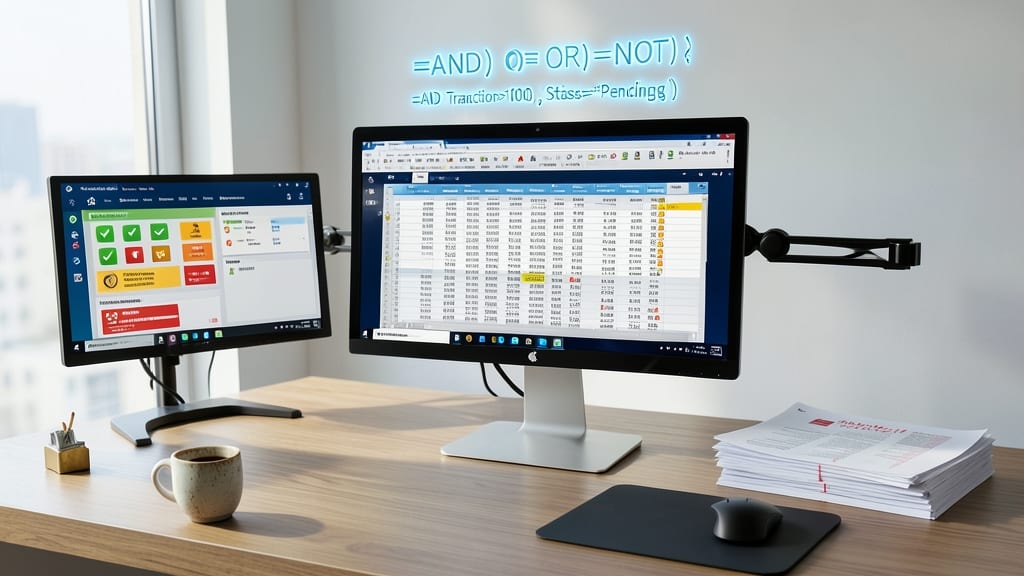
When you need to filter data based on multiple conditions—like finding high-risk transactions and overdue payments—AND, OR, and NOT become your secret weapons. These logical functions let you layer conditions to create precise filters, turning messy datasets into clear insights.

Use AND to require all conditions (e.g., =AND(A2>100, B2="High")), OR for any condition (e.g., =OR(C2="Approved", D2="Pending")), and NOT to exclude values (e.g., =NOT(E2="Error")). Combine them to build complex rules—like identifying overdue invoices not marked as paid. Excel 2013’s logical operators work seamlessly with other functions (e.g., nested in IF or SUMIFS).

Perfect for auditors, risk managers, or anyone sifting through layered criteria—these functions cut through noise to highlight exactly what matters. ✨